A direction-finding (DF) receiver estimates the bearing of an emitter by comparing the signals of several antennas. Most model-based estimators, from the beamscan to MUSIC, do so by matching the received data against the array response vector, the complex response of the array to a plane wave from a given direction. On a small drone the antennas sit a few centimetres from carbon plates, arms, landing legs, a battery and their own feed cables, all of them comparable in size to the wavelength. The airframe becomes part of the array. This post quantifies, in simulation, how far the installed response departs from the textbook one, what that does to bearings and to the position of an emitter, and which calibration is good enough to recover it.
The array response vector and the array manifold
For an array of elements, the array response vector collects the complex voltages at the ports for a unit plane wave arriving from azimuth and elevation (it is also called the steering vector). The array manifold is the set of all of them,
a two-dimensional surface in . The textbook model assumes identical, uncoupled elements in free space, so that the response differs between elements only by the geometric phase,
with the position of element , the unit vector toward the emitter, the wavenumber and a pattern common to all elements. Installed on a platform, element has its own embedded pattern, which includes the coupling to the other elements and the field scattered by everything nearby. The installed response vector is the vector of those embedded patterns, and it is a property of the array and the airframe together.
MUSIC [1] makes the dependence explicit. With the noise subspace of the sample covariance matrix, the bearing estimate is the direction whose response vector is most nearly orthogonal to it,
The search runs over whichever response vectors the receiver holds: a formula, or a table of measured or simulated response vectors, a sampled version of the manifold. If they are not those of the installed array, the estimate is wrong regardless of noise.
A drone in the simulator
The test case is four vertical half-wave dipoles on a square of side ( cm) at GHz, hanging below the body of a -class quadcopter with their tops cm from it. The airframe is modelled as a perfectly conducting wire grid (body plates, arms, motors, landing legs) and solved with the method of moments in NEC-2 [2]. The installed response vectors are computed in receive mode, as the port voltages for plane waves from every direction, and stored in the effective aperture distribution function (EADF) form [3], a Fourier series in azimuth that gives the response and its derivative at any angle.
Fig. 1 shows what the airframe does to an incoming wave. It is a snapshot, seen from above, of the vertical electric field (the component the dipoles respond to) in the horizontal plane through the four dipoles, for an emitter at azimuth 25° and elevation −10°. Without the drone, the wavefronts are straight, evenly spaced bands moving across the array, and the phase difference between any two dipoles depends only on their spacing and the direction of arrival. That is the textbook model, and it is what the estimator inverts to obtain a bearing. Under the drone, the field at the dipoles is the incident wave plus the waves scattered by the body, the legs and the other dipoles, and the bands bend and break up around the airframe.
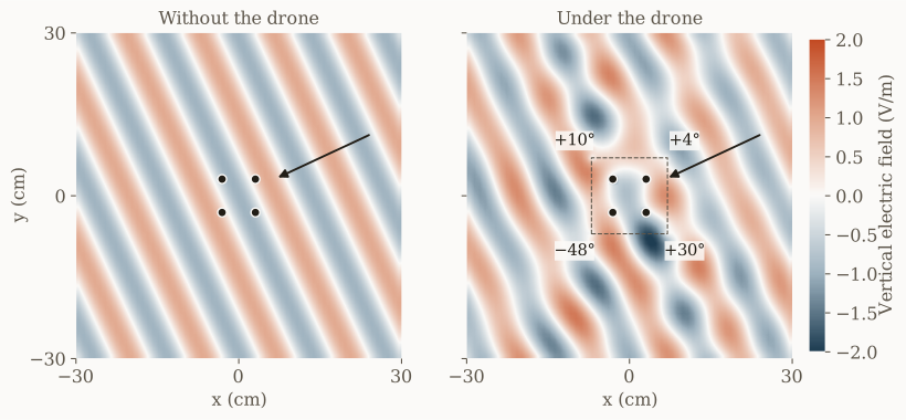
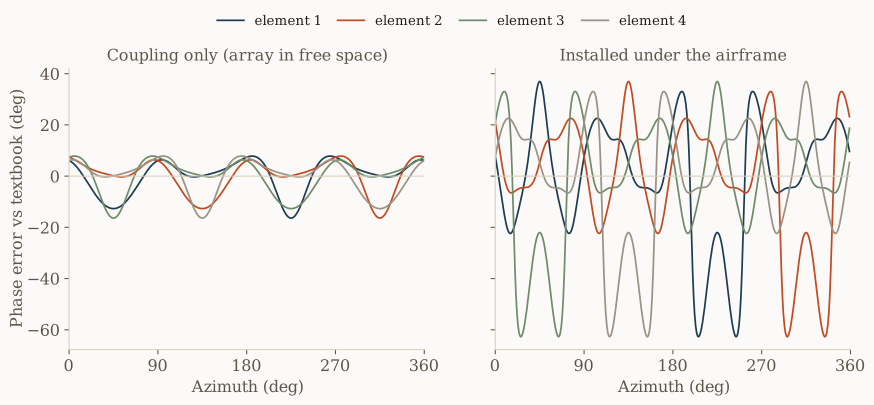
For this direction the phase errors at the four dipoles are +4°, +10°, −48° and +30°, where the textbook model assumes zero. Those phases are what the estimator reads. Fig. 2 separates the two mechanisms. Coupling between the dipoles alone shifts the phase of each element by up to about 15°; the airframe adds up to about 60°, with a different dependence on azimuth for each element.
Bearings from the textbook and the installed response
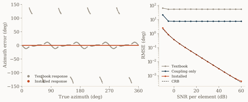
Fig. 3 compares MUSIC with the two sets of response vectors on the same data, one emitter, a signal-to-noise ratio (SNR) of dB per element and snapshots unless stated otherwise. With the installed response vectors the estimator reaches the Cramér–Rao bound (CRB) [4], 0.010°, slightly below the 0.013° of the textbook array. The scattered field makes the response vector change faster with direction (it needs more than twice as many Fourier terms in azimuth), which raises the information available about the angle. The airframe does not reduce that information; it changes the response that carries it.
With the textbook response vectors the RMSE is 57°. The error is not random: for a given direction it is the same in every trial. About % of directions are within 10° of the truth, another % carry a bias of 10° to 20°, and the remaining % are reported 115° to 140° away. The emitter at 25° in Fig. 1 is reported at 153°; with the installed response it is reported at 25.0°. A response that accounts for coupling but not for the airframe still leaves 8° RMSE. Because the error is deterministic, a higher SNR or more snapshots do not reduce it: the RMSE curve flattens into a floor set by the model, not by the noise.
Why the errors are large: the ambiguity margin
A bias of a few degrees is the expected effect of a model error. The jumps of more than 100° come from the structure of the manifold. Define the ambiguity margin at a direction as one minus the largest normalized correlation with any response vector more than 30° away in azimuth. A margin close to zero means that two distant directions are nearly indistinguishable, and a small model error is enough to swap them. Table 1 lists the worst case over azimuth.
| Elevation | −5° | −10° | −20° | −30° | −40° |
|---|---|---|---|---|---|
| Textbook array | < 0.001 | < 0.001 | 0.004 | 0.022 | 0.067 |
| Installed array | 0.017 | 0.030 | 0.045 | 0.019 | 0.005 |
Table 1: Ambiguity margin (worst case over azimuth).
A square of side is ambiguous toward the horizon: there the inter-element phase approaches , and its two signs can no longer be told apart. Processing with the textbook response therefore fails near the horizon, where most ground emitters lie when seen from a drone at a few kilometres. On this airframe the installed array is instead nearly ambiguous at steep elevation, so any error in a calibration table shows up there. The ambiguity margin can be computed before anything is built and is a useful figure of merit for placement.
Shift invariance does not survive the airframe
ESPRIT [5] needs no table of response vectors. It assumes two identical subarrays displaced by a known vector, so that for every direction. That requires each element of a pair to see the same surroundings, displaced by . A symmetric installation does not provide it: mirror or rotational symmetry maps an element’s surroundings onto another’s reflected or rotated, not translated. For the emitter at 25° the two pairs along should both show a phase step of 161°; on the drone they show 155° and −121°, and ESPRIT reports 157°. For thin dipoles, coupling alone is very nearly a linear transformation of the textbook response [7], and one interpolation matrix [6] removes it to a residual of % (relative Frobenius norm over all azimuths at −10° elevation). The airframe is not: the best single matrix leaves a residual of % in the same measure, and the corrected ESPRIT is worse than the uncorrected one. On an installed array, table-based estimators are the practical choice. Search-free processing remains possible through manifold separation [8], which applies root-MUSIC to the Fourier representation of any array.
Realistic drones and the choice of calibration
A real drone differs from its CAD model. Sixteen simulated drones add element position errors of mm, length errors of %, a body gap tolerance of mm, a battery, carbon propellers at random angles, a misalignment of ±1° between array and inertial unit, and residual receiver gain and phase errors of dB and 2°; half of them also carry unchoked coaxial feed cables. Each drone is processed with five sets of response vectors: the textbook model; the array calibrated on its own in a chamber, then installed; a simulation of the nominal airframe; a flight calibration made of yaw rotations at five altitudes (elevations −5° to −40°) with a beacon at a known position, sampled every 5° in azimuth at dB SNR per point, with 0.3° heading error and the propellers in a different position; and, as a reference, the drone’s exact installed response. Elevation is unknown to the estimator and searched jointly with azimuth.
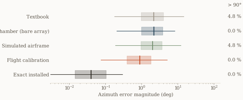
Fig. 4 shows the drones without feed cables. Textbook, chamber and simulated-airframe responses all give a median error near 2°; the textbook and simulated ones also produce errors above 90° in about % of directions. Flight calibration gives 0.9° median and 5.1° at the 95th percentile, with no gross errors. With unchoked feed cables, the textbook, chamber and simulated-airframe responses produce gross errors in to % of directions, while flight calibration stays at 0.8° median. Introducing the unmodelled effects one at a time shows that the feed cables dominate, followed by millimetre-level element tolerances; the battery and the channel errors matter little. A simulation of the airframe is the right tool to choose a placement and to anticipate where the array is fragile, but at this level of detail it is not a substitute for calibrating the built drone.
From bearings to a position
Bearing errors become position errors when bearings from several drones are combined. Fig. 5 places three drones at m altitude, to km from a ground emitter, with random headings, and intersects their bearings by least squares. The median miss distance is about km with the textbook response, m with the chamber-calibrated array, m with the simulated airframe, m with flight calibration and m with the exact response. The fix does not always reveal its own error: in the example of Fig. 5, the three bearings from the chamber-calibrated array pass within about m of their intersection, which lies m from the emitter. The agreement of the bearings is therefore no check on the calibration. A single drone taking bearings along a km leg behaves similarly, with medians from several kilometres for the textbook response to below m with flight calibration.
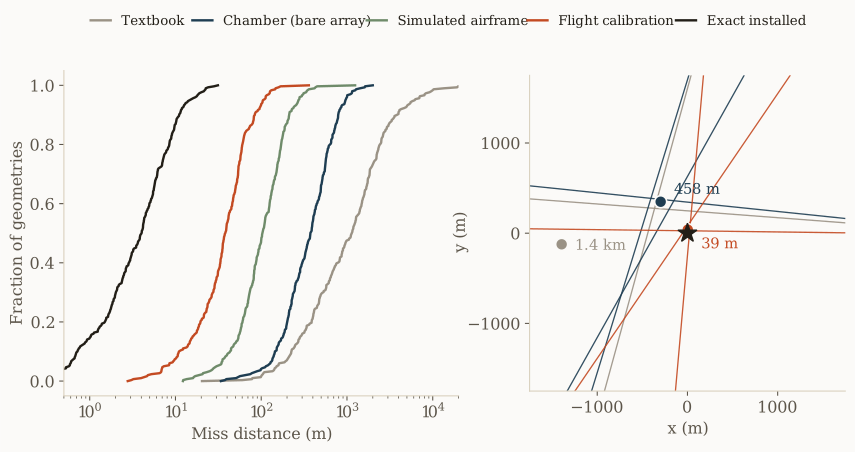
Table 2 collects the results for the five sets of response vectors.
| Response vectors | Median | 95th pct. | Errors > 90° | Errors > 90°, with feed cables | Miss distance, 3 drones |
|---|---|---|---|---|---|
| Textbook | 2.2° | 14.7° | 4.8 % | 11.3 % | 1.1 km |
| Chamber (bare array) | 2.2° | 8.3° | 0 % | 11.1 % | 370 m |
| Simulated airframe | 2.0° | 12.2° | 4.8 % | 14.6 % | 100 m |
| Flight calibration | 0.9° | 5.1° | 0 % | 0.1 % | 38 m |
| Exact installed | 0.04° | 0.3° | 0 % | 0 % | 4 m |
Table 2: Azimuth error and median miss distance per set of response vectors; drones without feed cables unless stated. SNR 30 dB, elevation −5° to −40°.
The gross-error rates in Table 2 are lower than the % of Fig. 3 because they average over elevations from −5° to −40°. Near the horizon (−5° to −10°), where the textbook array is ambiguous, the textbook response produces gross errors in to % of directions on these drones.
Limitations
The results come from one airframe, one frequency, one four-element array and a wire-grid model that treats carbon fibre as a perfect conductor. The emitter is single, and ground reflection is not modelled. The flight calibration is simulated, including its noise and the motion of the propellers, but it has not been flown. The trends are consistent across the sixteen drones; the numbers are not a substitute for a measurement.
Summary
Mounted on a small drone, an array no longer has the response of the textbook model or of its own chamber measurement. The angular information is still there, and with the installed response the estimator reaches the CRB. With any other response the bearing error is deterministic, does not average out, and includes gross errors wherever the ambiguity margin is small. Feed cables and millimetre tolerances are enough to spoil a table derived from the CAD model. Calibration on the built drone, in azimuth and elevation, is what turns the estimator’s precision into accuracy. The next step is a measurement on a real frame; if you work on DF for small platforms and would like to compare notes, I would be glad to hear from you.
References
[1] R. O. Schmidt, “Multiple emitter location and signal parameter estimation,” IEEE Transactions on Antennas and Propagation, vol. 34, no. 3, pp. 276–280, 1986.
[2] G. J. Burke and A. J. Poggio, “Numerical Electromagnetics Code (NEC)—Method of Moments,” Lawrence Livermore National Laboratory, Tech. Rep. UCID-18834, 1981.
[3] M. Landmann and G. Del Galdo, “Efficient antenna description for MIMO channel modelling and estimation,” in Proc. 7th European Conference on Wireless Technology, Amsterdam, 2004, pp. 217–220.
[4] P. Stoica and A. Nehorai, “Performance study of conditional and unconditional direction-of-arrival estimation,” IEEE Transactions on Acoustics, Speech, and Signal Processing, vol. 38, no. 10, pp. 1783–1795, 1990.
[5] R. Roy and T. Kailath, “ESPRIT—Estimation of signal parameters via rotational invariance techniques,” IEEE Transactions on Acoustics, Speech, and Signal Processing, vol. 37, no. 7, pp. 984–995, 1989.
[6] B. Friedlander, “The root-MUSIC algorithm for direction finding with interpolated arrays,” Signal Processing, vol. 30, no. 1, pp. 15–29, 1993.
[7] B. Friedlander and A. J. Weiss, “Direction finding in the presence of mutual coupling,” IEEE Transactions on Antennas and Propagation, vol. 39, no. 3, pp. 273–284, 1991.
[8] F. Belloni, A. Richter, and V. Koivunen, “DoA estimation via manifold separation for arbitrary array structures,” IEEE Transactions on Signal Processing, vol. 55, no. 10, pp. 4800–4810, 2007.